Applying VictoriaMetrics Stream Aggregation for Metrics
Community VM Stream Aggregation Capability Analysis and Issues
VictoriaMetrics Open-Source Project Native Capabilities
Stream aggregation in the VictoriaMetrics project was integrated into vmagent starting from version 1.86. For details, refer to: https://github.com/VictoriaMetrics/VictoriaMetrics/issues/3460 From the source code analysis, the stream aggregation capability looks like this:
The core computation code is described in the pushSample function:
| |
General Application Analysis of Stream Aggregation
First, let’s look at the time series chart after stream aggregation:
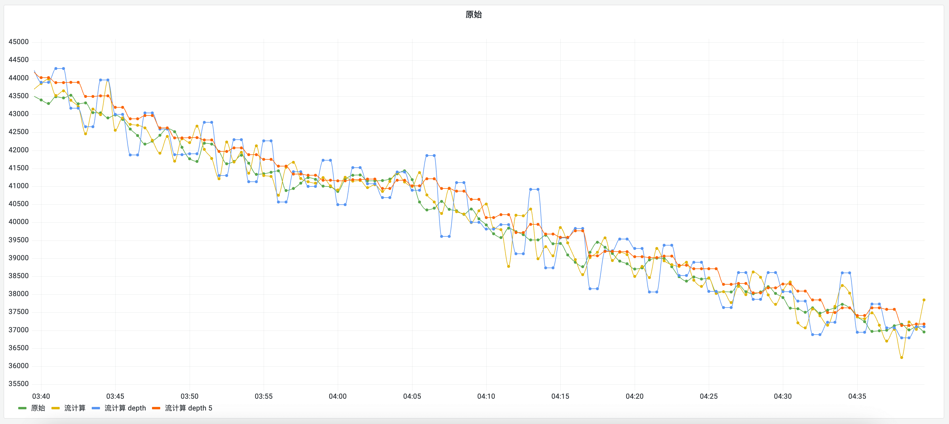
Now, let’s look at the theoretical form of time series data:

The ideal stream aggregation form based on the theoretical model:

The stream aggregation form in actual conditions:

Common Issues with Native Stream Aggregation
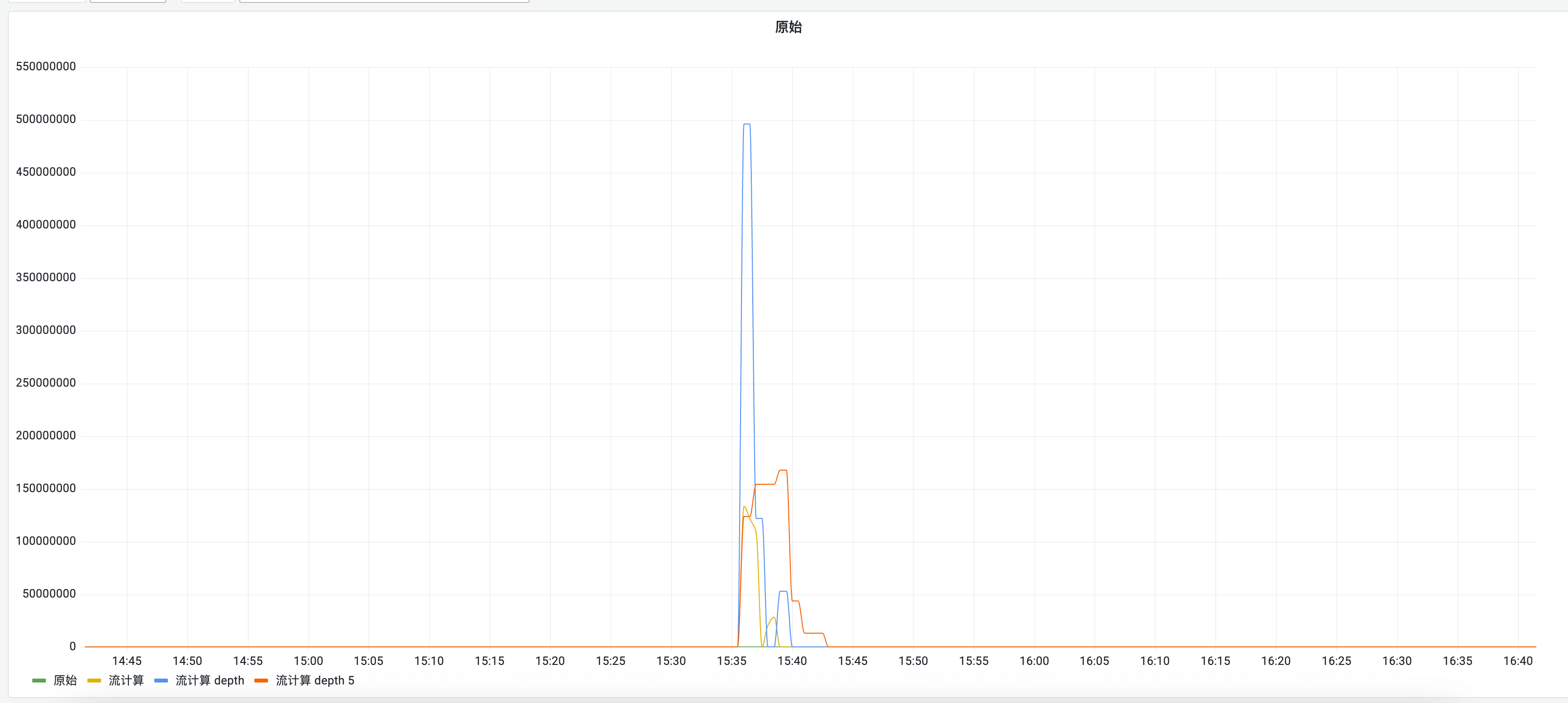
Collection Gap Problem
In the real world, things are more harsh: collection gaps are unavoidable for various reasons—network issues, performance problems on the collected services, etc.
 The impact of high-precision stream aggregation gap issues in large-number calculations is extreme:
Computing Architecture for Massive Data
Stream aggregation doesn’t save historical data details, so performance is excellent. But even the best-performing service has single-point limits. When dealing with data volumes that a single point cannot handle, distributed computing architecture introduces a series of problems:
Is vmagent’s built-in collection capability usable?
In actual testing, enabling vmagent shard + replica collection combined with real-time stream aggregation significantly increased resource usage. At very large scales, continuous collection gaps occurred frequently, worsening the calculation result differences caused by gaps.
 Reference architecture diagram:

Which compute node should each Sample’s data be assigned to?
How to solve the problem of same-dimension metric sets computed by multiple nodes having different result values within the same time window, causing later values to be discarded? (Triggering out-of-order metric handling logic)

Resource balancing in distributed computing?
After inserting a task ID to solve compute node differentiation for same dimensions, how to handle the new dimension introduced?

Design and Implementation of a Distributed Stream Aggregation Gateway
After analyzing the problems encountered in current industry solutions combined with real scenarios in the previous section, this section addresses each problem specifically.
Through source code analysis, there are two key parts:
- Time window range:
| |
- Calculation window logic:
| |
From the source code analysis, the stream aggregation logic only performs simple periodic checks on the time window. There isn’t much handling for inflated calculated values caused by delayed arrival of incoming metrics due to various reasons.
At this point, we need a frontend module to solve some problems. Since vmgateway is an enterprise component, we developed our own distributed stream aggregation gateway vm-receive-route.
Problems Addressed by the Distributed Stream Aggregation Gateway

Asynchronous Processing
Most remote write projects do synchronous forwarding. For example, prometheus-kafka-adapter waits for kafka to complete data production logic before completing the entire write process and processing the next batch of remote write data.
However, stream computation has window constraints on data processing. If synchronous logic blocks here, performance is affected, causing subsequent samples to be delayed. If delays miss the stream computation time window, calculation deviations occur. Therefore, asynchronous forwarding is the right approach here.

Time Window Filtering
Since the stream aggregation logic already compares the difference between new and old values on the time series, there’s no need to introduce an out-of-order algorithm.
The gateway only needs to cooperate with the stream aggregation logic’s time window to filter and discard samples.
This mainly solves the problem of Prometheus retries sending large backlogs of old samples affecting real-time calculation results, and also resolves the resource performance issues caused by Prometheus retries with large sample backlogs.

Dimension Control
Since the stream aggregation component inserts a node ID into each aggregated time series to distinguish labels. However, as nodes scale horizontally, this label’s dimensions also increase. We need a way to control dimensions, while simultaneously distributing time series by dimension ID to different nodes for processing. Later, we designed a dual hashmod scheduling algorithm to solve these problems.
By moving the taskid labeling capability to the gateway, we can ignore the impact of horizontal scaling node count on the task ID dimension:

Dual Hashmod Scheduling
Omitted for brevity.
Backend Service Migration for Failures
Omitted for brevity.
Program Flow Logic Diagram

Production Environment Architecture Diagram

Record Rule Dimension Task Generator
Stream aggregation is a technique for real-time processing and analyzing large data streams. Its main purpose is to extract valuable information from high-speed, continuous data streams, such as: calculating averages, sums, maximums, minimums, etc. Stream aggregation is typically performed in memory to maintain low latency and high throughput.
The implementation of stream aggregation typically includes the following key components:
- Data source and data sink: Define and monitor data streams such as logs, network packets, sensor data, splitting the data stream into multiple mini-batches.
- Window operations: Data streams are divided into fixed or sliding windows. Data within each window undergoes predefined aggregation operations.
- Aggregation functions: Various operations on data within windows, such as count, sum, average, max/min, etc.
- Output: Output or store aggregation results for further processing or real-time data visualization.
In metric stream aggregation, this capability efficiently reduces dimensions for a single metric. However, in reality, describing complex scenarios requires combining multiple metrics with functions.
Stream aggregation can efficiently solve the following aggregation problem of filtering the req_path field:
- Before aggregation:
| |
- After aggregation:
| |
But what we ultimately want to display is the success rate for a specific target:
| |
We can use Prometheus’s Record Rule to directly compute aggregated scenario metrics.
| |
But Record Rule loads all dimension data of the metric a_http_req_total into memory. If the dimension count reaches a critical threshold, it triggers OOM. Even if not critical, the computation load increases with dimensions, delaying calculation results.
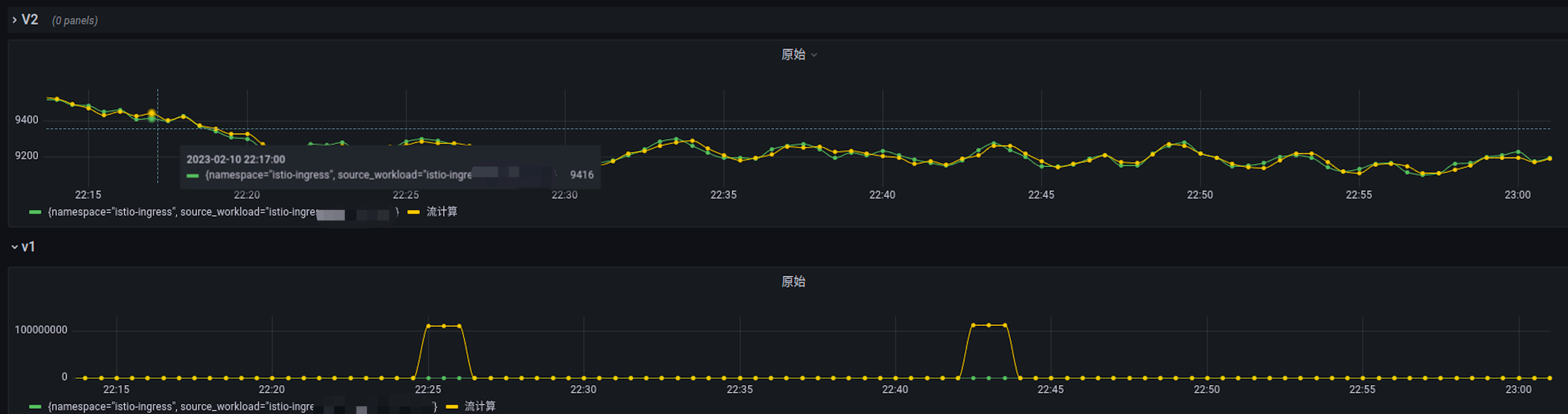
In actual production environments, istio_request_total QPS data could be delayed by 20 minutes.
Combining stream aggregation to reduce dimensions—from tens of millions of time series down to tens of thousands—only reduces delay from 20 minutes to 1-2 minutes.
Record Rule configuration after stream aggregation:
| |
By analyzing the source code of the Rule module, we can create more granular configurations:
| |
This way, we can split queries by specific dimension labels to achieve concurrent processing for generating the same new metrics.
The problem is that most production dimension labels are dynamically changing. How do we dynamically generate such dimension-split queries for concurrent Record Rule processing? We need a label metadata management system to track and manage label dimension metadata.
We implemented a small metadata watch module and rule build module to solve this problem.
The configuration for this ruler-handle-process component is:
| |
ruler-handle-process watches the dimension combinations response_code, namespace, source_workload_namespace, destination_workload_namespace, destination_service_name, cluster, reporter under the metric name "istio_requests_total" to generate a set of Record Rule rules.
Combined with the Rule component for concurrent computation, we can reduce computation latency to seconds.
| |
Stream Aggregation Architecture Combinations in the Monitoring Platform
Using community open-source programs and our self-developed components, we can combine different solutions for different collection scales to handle high-dimensional data at various levels.
Stream Aggregation for Tens of Thousands of Single Metrics

Computational Aggregation for Tens of Thousands of Multi-Metrics

Stream Aggregation for Millions+ of Single Metrics
Scenario-Based Computational Aggregation for Millions+ of Metrics
